Parameter management

Some prerequisites & basic definitions

import numpy as np
import pandas as pd
import datetime as dt
pd.set_option("mode.chained_assignment", None)
# in case eao is not installed
import os
import sys
# in case eao is not installed, set path
myDir = os.path.join(os.getcwd(), '../..')
sys.path.append(myDir)
addDir = os.path.join(os.getcwd(), '../../../..')
sys.path.append(addDir)

import eaopack as eao

import matplotlib.pyplot as plt
%matplotlib inline

Load sample portfolio (and the timegrid)

The portfolio comes prefefined in a JSON. Let us have a look.

timegrid = eao.serialization.load_from_json(file_name='timegrid.json')
portf    = eao.serialization.load_from_json(file_name='portfolio_simple_start.json')
eao.network_graphs.create_graph(portf)

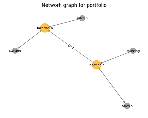
As we can see. the portfolio is a simple setup with a sourcing possibility and two sales contracts at two locations. For flexibility there is a storage (which we will manipulate in the following)

Looking at parameters and setting them to new values

As the next step we look at the parameters that define the portfolio. To this end, EAO provides three routines:

• eao.io.get_params_tree - to retrieve parameters as a dict and the paths to the parameters. To be used mainly with assets & portfolios

• get_param - to get parameter values using the path

• set_param - to change the parameters

[params, param_dict] = eao.io.get_params_tree(portf)
for p in params:
    print(p)

__class__
['assets', 0, '__class__']
['assets', 0, 'asset_type']
['assets', 0, 'end']
['assets', 0, 'extra_costs']
['assets', 0, 'freq']
['assets', 0, 'max_cap']
['assets', 0, 'min_cap']
['assets', 0, 'name']
['assets', 0, 'nodes', 0, '__class__']
['assets', 0, 'nodes', 0, 'commodity']
['assets', 0, 'nodes', 0, 'name']
['assets', 0, 'nodes', 0, 'unit', '__class__']
['assets', 0, 'nodes', 0, 'unit', 'factor']
['assets', 0, 'nodes', 0, 'unit', 'flow']
['assets', 0, 'nodes', 0, 'unit', 'volume']
['assets', 0, 'periodicity']
['assets', 0, 'periodicity_duration']
['assets', 0, 'price']
['assets', 0, 'profile']
['assets', 0, 'start']
['assets', 0, 'wacc']
['assets', 1, '__class__']
['assets', 1, 'asset_type']
['assets', 1, 'end']
['assets', 1, 'extra_costs']
['assets', 1, 'freq']
['assets', 1, 'max_cap']
['assets', 1, 'min_cap']
['assets', 1, 'name']
['assets', 1, 'nodes', 0, '__class__']
['assets', 1, 'nodes', 0, 'commodity']
['assets', 1, 'nodes', 0, 'name']
['assets', 1, 'nodes', 0, 'unit', '__class__']
['assets', 1, 'nodes', 0, 'unit', 'factor']
['assets', 1, 'nodes', 0, 'unit', 'flow']
['assets', 1, 'nodes', 0, 'unit', 'volume']
['assets', 1, 'periodicity']
['assets', 1, 'periodicity_duration']
['assets', 1, 'price']
['assets', 1, 'profile']
['assets', 1, 'start']
['assets', 1, 'wacc']
['assets', 2, '__class__']
['assets', 2, 'asset_type']
['assets', 2, 'end']
['assets', 2, 'extra_costs']
['assets', 2, 'freq']
['assets', 2, 'max_cap']
['assets', 2, 'min_cap']
['assets', 2, 'name']
['assets', 2, 'nodes', 0, '__class__']
['assets', 2, 'nodes', 0, 'commodity']
['assets', 2, 'nodes', 0, 'name']
['assets', 2, 'nodes', 0, 'unit', '__class__']
['assets', 2, 'nodes', 0, 'unit', 'factor']
['assets', 2, 'nodes', 0, 'unit', 'flow']
['assets', 2, 'nodes', 0, 'unit', 'volume']
['assets', 2, 'periodicity']
['assets', 2, 'periodicity_duration']
['assets', 2, 'price']
['assets', 2, 'profile']
['assets', 2, 'start']
['assets', 2, 'wacc']
['assets', 3, '__class__']
['assets', 3, 'asset_type']
['assets', 3, 'costs_const']
['assets', 3, 'costs_time_series']
['assets', 3, 'efficiency']
['assets', 3, 'end']
['assets', 3, 'freq']
['assets', 3, 'max_cap']
['assets', 3, 'min_cap']
['assets', 3, 'name']
['assets', 3, 'nodes', 0, '__class__']
['assets', 3, 'nodes', 0, 'commodity']
['assets', 3, 'nodes', 0, 'name']
['assets', 3, 'nodes', 0, 'unit', '__class__']
['assets', 3, 'nodes', 0, 'unit', 'factor']
['assets', 3, 'nodes', 0, 'unit', 'flow']
['assets', 3, 'nodes', 0, 'unit', 'volume']
['assets', 3, 'nodes', 1, '__class__']
['assets', 3, 'nodes', 1, 'commodity']
['assets', 3, 'nodes', 1, 'name']
['assets', 3, 'nodes', 1, 'unit', '__class__']
['assets', 3, 'nodes', 1, 'unit', 'factor']
['assets', 3, 'nodes', 1, 'unit', 'flow']
['assets', 3, 'nodes', 1, 'unit', 'volume']
['assets', 3, 'periodicity']
['assets', 3, 'periodicity_duration']
['assets', 3, 'profile']
['assets', 3, 'start']
['assets', 3, 'wacc']
['assets', 4, '__class__']
['assets', 4, 'asset_type']
['assets', 4, 'block_size']
['assets', 4, 'cap_in']
['assets', 4, 'cap_out']
['assets', 4, 'cost_in']
['assets', 4, 'cost_out']
['assets', 4, 'cost_store']
['assets', 4, 'eff_in']
['assets', 4, 'end']
['assets', 4, 'end_level']
['assets', 4, 'freq']
['assets', 4, 'inflow']
['assets', 4, 'max_store_duration']
['assets', 4, 'name']
['assets', 4, 'no_simult_in_out']
['assets', 4, 'nodes', 0, '__class__']
['assets', 4, 'nodes', 0, 'commodity']
['assets', 4, 'nodes', 0, 'name']
['assets', 4, 'nodes', 0, 'unit', '__class__']
['assets', 4, 'nodes', 0, 'unit', 'factor']
['assets', 4, 'nodes', 0, 'unit', 'flow']
['assets', 4, 'nodes', 0, 'unit', 'volume']
['assets', 4, 'periodicity']
['assets', 4, 'periodicity_duration']
['assets', 4, 'price']
['assets', 4, 'profile']
['assets', 4, 'size']
['assets', 4, 'start']
['assets', 4, 'start_level']
['assets', 4, 'wacc']

Looking at the parameter tree, note that we extracted the whole tree of parameters in the portfolio. Each entry is a list, that points downwards into the nested object (portfolio –> asset, –> …)

To access the parameter, we can use any of those entries. Let us concentrate on the storage (asset no. 4):

param_dict['assets'][4]

{'__class__': 'Asset',
 'asset_type': 'Storage',
 'block_size': None,
 'cap_in': 30,
 'cap_out': 30,
 'cost_in': 0.2,
 'cost_out': 0.2,
 'cost_store': 0.0,
 'eff_in': 1.0,
 'end': None,
 'end_level': 5,
 'freq': None,
 'inflow': 0.0,
 'max_store_duration': None,
 'name': 'storage',
 'no_simult_in_out': False,
 'nodes': [{'__class__': 'Node',
   'commodity': None,
   'name': 'location b',
   'unit': {'__class__': 'Unit',
    'factor': 1.0,
    'flow': 'MW',
    'volume': 'MWh'}}],
 'periodicity': None,
 'periodicity_duration': None,
 'price': None,
 'profile': None,
 'size': 48,
 'start': None,
 'start_level': 5,
 'wacc': 0.0}

Now, get direct access via tree entries, e.g. the fill level on start up

print(eao.io.get_param(portf, ['assets', 4, 'start_level']))

5

Going via the complete portfolio is one way. However, it is also possible to directly go via specific assets:

print(eao.io.get_param(portf.get_asset('sales b'), ['price']))

price sales b

Let us manipulate the fill level. Note that this could also be done by diving directly into the object …

portf.get_asset('storage').start_level = 4
print(portf.get_asset('storage').start_level)

4

… but setting parameters this way is actually relatively insecure, since this circumvents proper initialization. Therefore, it is better to use the set_param routine:

portf = eao.io.set_param(portf,['assets', 4, 'start_level'], 6 )
print(portf.get_asset('storage').start_level)

6

This routine properly extracts parameters using the serialization machinery and re-initiates the objects. Therefore, all tests are called.

Let us take a look by setting an invalid parameter. In this case we set the storage size to a value which is smaller than the initial fill level:

try:
    portf = eao.io.set_param(portf, ['assets', 4, 'size'], 1.)
except Exception as error:
    print('Not possible')
    pass

Not possible

Sample: Looping different parameters

Here we do a simple loop on the storage size to demonstrate how to manipulate parameters for parameter studies or how to react to live data

# sample prices
prices = {'price sourcing': 5.*np.sin(np.linspace(0.,6., timegrid.T)),
         'price sales a' : np.ones(timegrid.T)*2.,
         'price sales b' : 5.+5.*np.sin(np.linspace(0.,6., timegrid.T))  }

Current storage size

print(eao.io.get_param(portf, ['assets', 4, 'size']))
print(eao.io.get_param(portf, ['assets', 4, 'nodes', 0,'unit','volume']))

48
MWh

storage_sizes = range(10, 150, 5)
values = [] # collect results

for my_size in storage_sizes:
    portf = eao.io.set_param(portf, ['assets', 4, 'size'], my_size )
    optim_problem  = portf.setup_optim_problem(timegrid = timegrid, prices=prices)
    result         = optim_problem.optimize()
    values.append(result.value)
# output = eao.io.extract_output(portf, optim_problem, result)

fig = plt.figure(figsize = (12,3))
plt.bar(storage_sizes, values, width = 4)
plt.ylim((6000, 7000))
plt.xlabel('storage size')
plt.ylabel('total portfolio value')
plt.show()

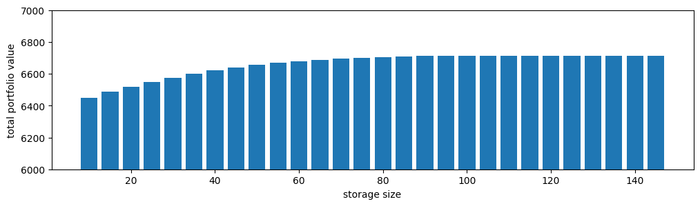
This is just for demonstration purpose. However - neat to see how the value add of extra storage size decreases.